Analyze a spatial section without writing code

Open a Xenium, Visium or CosMx run, put squidpy and scanpy through point-and-click forms, and watch every cell redraw over the tissue image. Each step is recorded as it happens, and the whole session saves to one file that reopens in a browser with nothing running behind it.

$ docker run -d -p 8080:8888 \
    -v "$(pwd)/data":/data \
    -e SDS_DATA_DIR=/data \
    public.ecr.aws/cirrobio/spatial-data-studio:v1

$ open http://localhost:8080 # your data, under /data

$ npm install # at the repo root$ ./run.sh --test # :8000 and :5173$ ./stop.sh # stops both

One image holds the SPA and the backend, and the folder you mount holds inputs, checkpoints and snapshots together — so the published build is the whole install, with nothing to clone and nothing to compile. Memory limits and the rest of the environment are in Run with Docker; running from a clone is in the development guide; the workspace is further down this page. To see it with nothing installed at all, the live demos are the real viewer running in your browser.

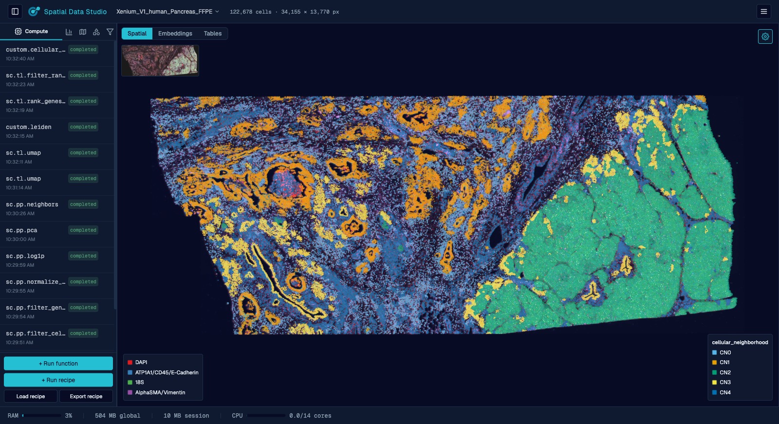
The spatial canvas showing a Xenium ovarian-cancer section, each cell colored by its cellular neighborhood, over the morphology image, with the left panel open on the Compute history tab. — A whole Xenium ovarian-cancer section — about 400,000 cells — colored by cellular neighborhood, over the morphology image. The left panel is on the Compute tab, which is the history of everything that produced what you are looking at. The user guide walks through each panel.

The unit of work

How an analysis moves

You pick a function, fill in a form built from that function's own signature, and it runs against the object in memory. Nothing is copied and nothing is versioned away: the analysis adds its columns, embeddings and graphs to the object you already have, and appends one entry to the session's history. What the canvas can color by grows as you go.

One function, then the file it all ends up in. The top row is the loop you spend the day in; the bottom row is what leaves the machine. The checkpoint is one file rather than a folder because that is what a browser can read a few kilobytes out of — opening a 438 MB checkpoint and coloring by a gene costs under a megabyte. The checkpoint format has the layout; DESIGN.md has the reasoning.

Every step is on the record

The Compute tab is the session's history: each function that ran, with its parameters and timing. It travels inside a saved file, so reopening one shows how the data got that way — including in the no-backend viewer.

Recipes for the usual path

Curated multi-step workflows — preprocess, cluster, annotate, neighborhood analysis — run in one click, or stage step by step so you can edit the parameters before each one goes.

Annotate and subset

Draw regions on the canvas, label the cells inside them, and carry a selection into a subset that becomes the object the next analysis runs on. Labels are obs columns like any other, so everything else can color by them.

Figures you can publish

Every plot the session drew is collected in a grid and downloads as SVG, PDF or PNG. A snapshot renders the current canvas as a vector PDF — points as vectors, image as raster — with the provenance embedded in the file.

Loading data

Point it at the folder the instrument wrote

A reader's own options are its own fields: whether Xenium reads transcripts, cell boundaries or the morphology image is a set of toggles, so you load exactly what you are going to use and leave the rest on disk. Large sections take a while to read, and the reader's log streams while it works.

Anything SpatialData can read is available, because the app does not hardcode a list of functions or formats — it reflects the installed libraries and builds the forms from what it finds. Adding a library means one catalog entry, not one entry per function.

User guide → Load your data

Xenium 10x · imaging-basedVisium, Visium HD 10x · sequencing-basedCosMx NanoStringMERSCOPE Vizgen*.zarr, *.zarr.zip a store this app saved

Functions come from the libraries themselves: squidpy wholesale, scanpy and spatialdata-io through a curated catalog, plus the methods written for this app. Each one carries a citation and a link to its own documentation, and the picker refuses an entry that has neither. What the bundled methods do.

The AI assistant

An agent can drive the studio you are looking at

The backend speaks the Model Context Protocol, so an agent can load data, run analyses and recipes, restyle the display, label regions, subset and save — and can look at what it drew, since renders come back with a world-coordinate grid and an exact pixel-to-coordinate mapping.

It is not a second copy of the app. The agent joins the same per-session edit lock a person takes, shows up on the padlock as Claude (assistant) while it works, and hands control back when it is done. Every change it makes appears in your browser as it happens.

$ claude mcp add --transport http \ spatial-data-studio \ http://127.0.0.1:8000/api/mcp

From a clone, claude finds it on its own through .mcp.json. The endpoint is unauthenticated like the rest of the API, so expose the port only to people and processes you would let edit your sessions. User guide → Work with an AI assistant.

The data backend

Run it where the data is

Spatial data is big in a way that decides the architecture. One Xenium run is a few hundred thousand cells under a morphology image measured in gigabytes, and a project holds several of them. Downloading a section to look at it is the slow part of the work, and the laptop it lands on is usually the wrong machine to run the analysis on anyway.

So the app is built to be brought to the data instead. Cirro is the data platform it is built alongside: a workspace there runs a container image inside a project with that project's datasets already mounted, and this app ships as exactly one image. It opens on data nobody downloaded, with the workspace's CPU and memory doing the work, so a section too big for a laptop is only a bigger workspace.

A workspace is one running app, and that turns out to matter more than the machine size. Everyone in the lab opens the same URL. Whoever opens a session holds its edit lock; everyone else watches, and each analysis appears on their screens as it finishes rather than on a reload. What you are looking at stays yours — your gene, your channels, your corner of the section — while someone else drives. Cirro is the first backend built rather than the only shape allowed: the app holds no platform credential of its own, and each person signs in as themselves.

One project, one workspace, several people. The solid arrows are what the app does on its own, and they only read. The dashed ones are yours to take: publishing a finished checkpoint into the project, and someone else opening it. What each person's browser can see is what their own Cirro account can see — there is no shared account and no credential on the server.

Sign in as yourself

Sign-in is per browser, through Cirro's device-code flow: you open a link, sign in as you normally would, and the app never sees a password. The server holds no Cirro credential and needs no Cirro configuration, so several people share one running app without sharing an account.

Publishing is the one write

Saved checkpoints upload as a new dataset alongside the data rather than on top of it. The upload carries the viewer itself and an index of what is in it, so the resulting dataset opens as a browsable collection for anyone with access — no app, no install, no download.

Two people, one session

The padlock next to a session name says who holds it and who is on it, and names everyone in the room. Take an unlocked session, hand yours over, or rename yourself from the two-word name you arrived with. Watching costs nothing: display settings are per-browser and never enter the session.

None of this is required to use the app — it runs perfectly well as a local Docker container over a folder on your own disk, and the checkpoint it writes is a plain file you can put anywhere that serves HTTP range requests. User guide → Work in Cirro has the workspace image, the session-sharing rules and the upload flow; DESIGN.md §15 has the auth and credential scoping.